#Excel tip: Formula to cross check ledger transactions

This is a real time saver, and I hope it’s useful to someone else.

If you have a typical “ledger” type spread sheet, with columns, payments in, payments out and balance – based on the image above. Perhaps this has been entered manually, or perhaps it’s been OCR’d from paper, there could be errors in it, and it can take alot of time to manually check each number.

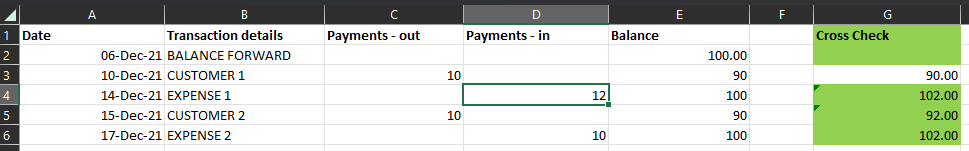
In the example above you can see there must be an issue with the value in Cell D4, since the Balance does not reflect the value. However, getting excel to highlight this error would allow you to manually check that one cell, not every value on the spreadsheet.

So, I added a new cell in G3 with the value =$E$2+SUM($D$3:D3)-SUM($C$3:C3) and copied this for each row in the spreadsheet. Then added a conditional formatting rule; of =$G1<>$E1

Which then highlights what the Balance should be for each row, and highlights it, if the balance is different to that stated. In this case, you can see that after a point, the projected Balance diverges from the stated balance, indicating the row at which an inaccuracy is present.

Correcting this value, and the projected balance now matches the stated balance, without having to check every single value on the spreadsheet.